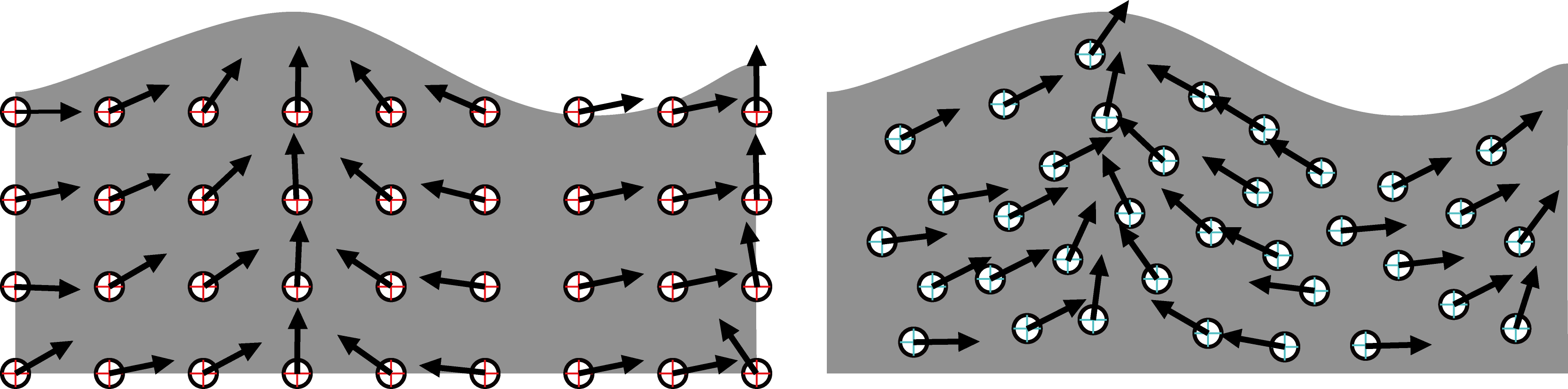
Figure 5.1: Left: Euler-like, Right: Lagrange-like
In the previous chapter, we explained how to create a fluid simulation using the grid method. In this chapter, we will use the particle method, which is another fluid simulation method, especially the SPH method, to express the movement of the fluid. Please note that there are some inadequate expressions as the explanation is given in a slightly chewed manner.
There are Euler's viewpoint and Lagrange's viewpoint as the method of observing the movement of fluid. Euler's viewpoint is to fix observation points on the fluid at equal intervals and analyze the movement of the fluid at the observation points. On the other hand, the Lagrange viewpoint is to float an observation point that moves along the flow of fluid and observe the movement of the fluid at that observation point ( see Fig. 5.1 ). Basically, the fluid simulation method using Euler's viewpoint is called the lattice method, and the fluid simulation method using Lagrange's viewpoint is called the particle method.
Figure 5.1: Left: Euler-like, Right: Lagrange-like
The method of calculating the derivative differs between the Euler perspective and the Lagrange perspective. First , the physical quantity * 1 expressed from Euler's point of view is shown below.
[* 1] Physical quantities refer to observable velocities and masses. In short, you can think of it as something that has a unit.
\phi = \phi (\overrightarrow{x}, t)
This means the physical quantity \ phi at the position \ overrightarrow {x} at time t . The time derivative of this physical quantity is
\frac{\partial \phi}{\partial t}
Can be expressed as. Of course, this is a derivative from Euler's point of view because the position of the physical quantity is fixed by \ overridearrow {x} .
[* 2] The movement of the observation point along the flow is called advection.
On the other hand, from the Lagrange perspective , the observation point itself is a function of time because it moves * 2 along the flow . Therefore, the observation point at \ overrightarrow {x} _0 in the initial state is at time t .
\overrightarrow{x}(\overrightarrow{x}_0, t)
Exists in. Therefore, the notation of physical quantities is also
\phi = \phi (\overrightarrow{x}(\overrightarrow{x}_0, t), t)
It will be. Looking at the current physical quantity and the amount of change in the physical quantity after \ Delta t seconds according to the definition of differentiation
\displaystyle \lim_{\Delta t \to 0} \frac{\phi(\overrightarrow{x}(\overrightarrow{x}_0, t + \Delta t), t + \Delta t) - \phi(\overrightarrow{x}(\overrightarrow{x}_0, t), t)}{\Delta t}
= \sum_i \frac{\partial \phi}{\partial x_i} \frac{\partial x_i}{\partial t} + \frac{\partial \phi}{\partial t}
  = \left( \left( \begin{matrix}u_1\\u_2\\u_3\end{matrix} \right)
    \cdot
    \left( \begin{matrix} \frac{\partial}{\partial x_1}\\\frac{\partial}{\partial x_2}\\\frac{\partial}{\partial x_3} \end{matrix} \right)
    + \frac{\partial}{\partial t}
    \right) \phi\\
= (\frac{\partial}{\partial t} + \overrightarrow{u} \cdot {grad}) \phi
It will be. This is the time derivative of the physical quantity considering the movement of the observation point. However, using this notation complicates the formula, so
\dfrac{D}{Dt} := \frac{\partial}{\partial t} + \overrightarrow{u} \cdot {grad}
It can be shortened by introducing the operator. A series of operations that take into account the movement of observation points is called Lagrange differentiation. At first glance, it may seem complicated, but in the particle method where the observation points move, it is more convenient to express the equation from a Lagrangian point of view.
A fluid can be considered to have no volume change if its velocity is well below the speed of sound. This is called the uncompressed condition of the fluid and is expressed by the following formula.
\nabla \cdot \overrightarrow{u} = 0
This indicates that there is no gushing or disappearance in the fluid. Since the derivation of this equation involves a slightly complicated integral, the explanation is omitted * 3 . Think of it as "do not compress the fluid!"
[* 3] It is explained in detail in "Fluid Simulation for Computer Graphics --Robert Bridson".
In the particle method, a fluid is divided into small particles and the movement of the fluid is observed from a Lagrangian perspective. This particle corresponds to the observation point in the previous section. Even if it is called the "particle method" in one word, many methods have been proposed at present, and it is famous
And so on.
First, the Navier-Stokes equation (hereinafter referred to as NS equation) in the particle method is described as follows.
  \dfrac{D \overrightarrow{u}}{Dt} = -\dfrac{1}{\rho}\nabla p + \nu \nabla \cdot \nabla \overrightarrow{u} + \overrightarrow{g}
  \label{eq:navier}
The shape is a little different from the NS equation that came out in the grid method in the previous chapter. The advection term is completely omitted, but if you look at the relationship between the Euler derivative and the Lagrange derivative, you can see that it can be transformed into this shape well. In the particle method, the observation point is moved along the flow, so there is no need to consider the advection term when calculating the NS equation. The calculation of advection can be completed by directly updating the particle position based on the acceleration calculated by the NS equation.
A real fluid is a collection of molecules, so it can be said to be a kind of particle system. However, it is impossible to calculate the actual number of molecules with a computer, so it is necessary to adjust it to a computable size. Each grain ( * 4 ) shown in Figure 5.2 represents a portion of the fluid divided by a computable size. Each of these grains can be thought of as having a mass m , a position vector \ overridearrow {x} , a velocity vector \ overridearrow {u} , and a volume V , respectively.
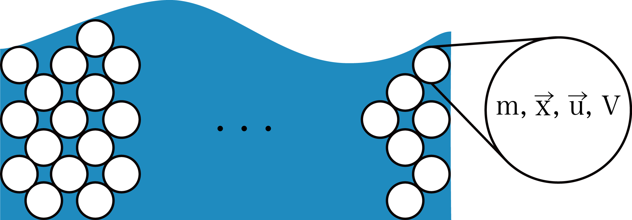
Figure 5.2: Fluid particle approximation
For each of these grains , the acceleration is calculated by calculating the external force \ overridearrow {f} and solving the equation of motion m \ overridearrow {a} = \ overridearrow {f} , and how in the next time step. You can decide whether to move to.
[* 4] Called'Blob'in English
As mentioned above, each particle moves by receiving some force from the surroundings, but what is that "force"? A simple example is gravity m \ overrightarrow {g}, but it should also receive some force from surrounding particles. These forces are explained below.
The first force exerted on a fluid particle is pressure. The fluid always flows from the higher pressure side to the lower pressure side. If the same amount of pressure is applied from all directions, the force will be canceled and the movement will stop, so consider the case where the pressure balance is uneven. As mentioned in the previous chapter, by taking the gradient of the pressure scalar field, it is possible to calculate the direction with the highest pressure rise rate from the viewpoint of your own particle position. The direction in which the particles receive the force is from the one with the highest pressure to the one with the lowest pressure, so take the minus and become-\ nabla p . Also, since particles have a volume, the pressure applied to the particles is calculated by multiplying-\ nabla p by the volume of the particles * 5 . Finally, the result --V \ nabla p is derived.
[* 5] Due to the uncompressed condition of the fluid, the integral of the pressure applied to the particles can be expressed simply by multiplying the volume.
The second force applied to fluid particles is viscous force. A viscous fluid is a fluid that is hard to deform, such as honey and melted chocolate. Applying the word viscous to the expression of the particle method, the velocity of a particle is easy to average the velocity of the surrounding particles . As mentioned in the previous chapter, the operation of averaging the surroundings can be performed using the Laplacian.
Expressing the degree of viscosity using the kinematic viscosity coefficient \ mu , it can be expressed as \ mu \ nabla \ cdot \ nabla \ overridearrow {u} .
Applying these forces to the equation of motion m \ overrightarrow {a} = \ overrightarrow {f} ,
m \dfrac{D\overrightarrow{u}}{Dt} = - V \nabla p + V \mu \nabla \cdot \nabla \overrightarrow{u} + m\overrightarrow{g}
Here, since m is \ rho V, it is transformed ( V is canceled).
\rho \dfrac{D\overrightarrow{u}}{Dt} = - \nabla p + \mu \nabla \cdot \nabla \overrightarrow{u} + \rho \overrightarrow{g}
Divide by both sides \ rho ,
\dfrac{D\overrightarrow{u}}{Dt} = - \dfrac{1}{\rho}\nabla p + \dfrac{\mu}{\rho} \nabla \cdot \nabla \overrightarrow{u} + \overrightarrow{g}
Finally, the coefficient of viscosity term \ dfrac {\ mu} {\ rho} in \ nu by introducing,
\dfrac{D\overrightarrow{u}}{Dt} = - \dfrac{1}{\rho}\nabla p + \nu \nabla \cdot \nabla \overrightarrow{u} + \overrightarrow{g}
Therefore, we were able to derive the NS equation mentioned at the beginning.
In the particle method, the particles themselves represent the observation points of the fluid, so the calculation of the advection term is completed by simply moving the particle position. In the actual calculation of the time derivative, infinitely small time is used, but since infinity cannot be expressed by computer calculation, the differentiation is expressed using sufficiently small time \ Delta t . This is called the difference, and the smaller \ Delta t , the more accurate the calculation.
Introducing the expression of difference for acceleration,
\overrightarrow{a} = \dfrac{D\overrightarrow{u}}{Dt} \equiv \frac{\Delta \overrightarrow{u}}{\Delta t}
It will be. So the velocity increment \ Delta \ overrightarrow {u} is
\Delta \overrightarrow{u} = \Delta t \overrightarrow{a}
And also for the position increment,
\overrightarrow{u} = \frac{\partial \overrightarrow{x}}{\partial t} \equiv \frac{\Delta \overrightarrow{x}}{\Delta t}
Than,
\Delta \overrightarrow{x} = \Delta t \overrightarrow{u}
It will be.
By using this result, the velocity vector and position vector in the next frame can be calculated. Assuming that the particle velocity in the current frame is \ overrightarrow {u} _n , the particle velocity in the next frame is \ overrightarrow {u} _ {n + 1} .
\overrightarrow{u}_{n+1} = \overrightarrow{u}_n + \Delta \overrightarrow{u} = \overrightarrow{u}_n + \Delta t \overrightarrow{a}
Can be expressed as.
Assuming that the particle position in the current frame is \ overridearrow {x} _n , the particle position in the next frame is \ overridearrow {x} _ {n + 1} .
\overrightarrow{x}_{n+1} = \overrightarrow{x}_n + \Delta \overrightarrow{x} = \overrightarrow{x}_n + \Delta t \overrightarrow{u}
Can be expressed as.
This technique is called the forward Euler method. By repeating this every frame, it is possible to express the movement of particles at each time.
In the previous section, we explained how to derive the NS equation in the particle method. Of course, these differential equations cannot be solved as they are on a computer, so some kind of approximation needs to be made. As a method, I will explain the SPH method that is often used in the CG field .
The SPH method was originally used for collision simulation between celestial bodies in astrophysics , but it was also applied to fluid simulation in CG by Desbrun et al. * 6 in 1996 . In addition, parallelization is easy, and the current GPU can calculate a large number of particles in real time. In computer simulation, it is necessary to discretize continuous physical quantities and perform calculations, and the method of performing this discretization using a function called a weight function is called the SPH method.
[*6] Desbrun and Cani, Smoothed Particles: A new paradigm for animating highly deformable bodies, Eurographics Workshop on Computer Animation and Simulation (EGCAS), 1996.
In the SPH method, each particle has an influence range, and the closer the particle is to other particles, the greater the influence of that particle. Figure 5.3 shows the extent of this effect .
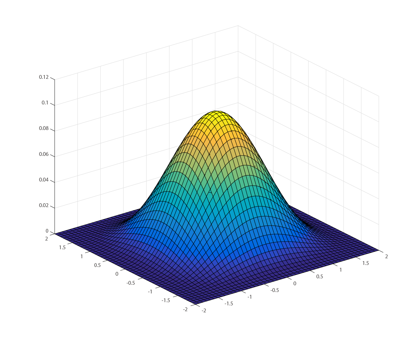
Figure 5.3: Two-dimensional weighting function
This function is called the weight function * 7 .
[* 7] Normally, this function is also called a kernel function, but it is called this function to distinguish it from the kernel function in Compute Shader.
Assuming that the physical quantity in the SPH method is \ phi , it is discretized as follows using a weighting function.
\phi(\overrightarrow{x}) = \sum_{j \in N}m_j\frac{\phi_j}{\rho_j}W(\overrightarrow{x_j} - \overrightarrow{x}, h)
N, m, \ rho, and h are the set of neighboring particles, the mass of the particles, the density of the particles, and the radius of influence of the weighting function, respectively. Also, the function W is the weighting function mentioned earlier.
Furthermore, partial differential operations such as gradient and Laplacian can be applied to this physical quantity, and the gradient is
\nabla \phi(\overrightarrow{x}) = \sum_{j \in N}m_j\frac{\phi_j}{\rho_j} \nabla W(\overrightarrow{x_j} - \overrightarrow{x}, h)
Laplacian
\nabla^2 \phi(\overrightarrow{x}) = \sum_{j \in N}m_j\frac{\phi_j}{\rho_j} \nabla^2 W(\overrightarrow{x_j} - \overrightarrow{x}, h)
Can be expressed as. As you can see from the equation, the physical quantity gradient and the Laplacian are images that apply only to the weighting function. The weight function W is different depending on the physical quantity to be obtained, but the explanation of the reason is omitted * 8 .
[* 8] It is explained in detail in "Basics of Physical Simulation for CG-Makoto Fujisawa".
The density of fluid particles is determined by using the formula of the physical quantity discretized by the weighting function.
\rho(\overrightarrow{x}) = \sum_{j \in N}m_jW_{poly6}(\overrightarrow{x_j} - \overrightarrow{x}, h)
Is given. Here, the weight function W to be used is given below.
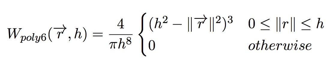
Figure 5.4: Poly6 weight function
Discretizing the viscosity term also uses the weighting function as in the case of density.
f_{i}^{visc} = \mu\nabla^2\overrightarrow{u}_i = \mu \sum_{j \in N}m_j\frac{\overrightarrow{u}_j - \overrightarrow{u}_i}{\rho_j} \nabla^2 W_{visc}(\overrightarrow{x_j} - \overrightarrow{x}, h)
Is expressed as. Where the weighting function Laplacian \ nabla ^ 2 W_ {visc} is given below.
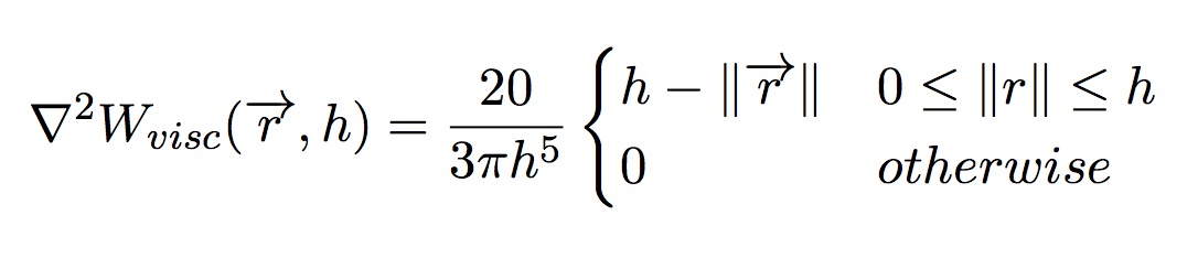
Figure 5.5: Laplacian of Viscosity weighting function
Similarly, the pressure term is discretized.
f_{i}^{press} = - \frac{1}{\rho_i} \nabla p_i = - \frac{1}{\rho_i} \sum_{j \in N}m_j\frac{p_j - p_i}{2\rho_j} \nabla W_{spiky}(\overrightarrow{x_j} - \overrightarrow{x}, h)
Where the gradient of the weighting function W_ {spiky} is given below.
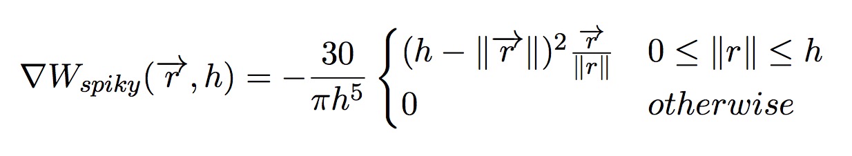
Figure 5.6: Gradient of Spiky weight function
At this time, the pressure of the particles is called the Tait equation in advance.
p = B\left\{\left(\frac{\rho}{\rho_0}\right)^\gamma - 1\right\}
It is calculated by. Where B is the gas constant. In order to guarantee incompressibility, Poisson's equation must be solved, but it is not suitable for real-time calculation. Instead, it is said that the SPH method * 9 is not as good at calculating the pressure term as the lattice method in terms of ensuring incompressibility approximately.
[* 9] The SPH method, which calculates pressure using the Tait equation, is specially called the WCSPH method.
Samples can be found under Assets / SPHFluid in this repository ( https://github.com/IndieVisualLab/UnityGraphicsProgramming ). Please note that in this implementation, speedup and numerical stability are not considered in order to explain the SPH method as simply as possible.
A description of the various parameters used in the simulation can be found in the comments in the code.
Listing 5.1: Parameters used for simulation (FluidBase.cs)
 1: NumParticleEnum particleNum = NumParticleEnum.NUM_8K; // Number of particles
 2: float smoothlen = 0.012f; // Particle radius
 3: float pressureStiffness = 200.0f; // Pressure term coefficient
 4: float restDensity = 1000.0f; // rest density
 5: float particleMass = 0.0002f; // particle mass
 6: float viscosity = 0.1f; // Viscosity coefficient
 7: float maxAllowableTimestep = 0.005f; // Time step width
 8: float wallStiffness = 3000.0f; // Penalty wall power
 9: int iterations = 4; // number of iterations
10: Vector2 gravity = new Vector2(0.0f, -0.5f);     // 重力
11: Vector2 range = new Vector2 (1, 1); // Simulation space
12: bool simulate = true; // Run or pause
13:
14: int numParticles; // Number of particles
15: float timeStep; // Time step width
16: float densityCoef; // Poly6 kernel density coefficient
17: float gradPressureCoef; // Pressure coefficient of Spiky kernel
18: float lapViscosityCoef; // Laplacian kernel viscosity coefficient
Please note that in this demoscene, the inspector sets a value that is different from the parameter initialization value described in the code.
Since the coefficient of the weight function does not change during simulation, it is calculated on the CPU side at the time of initialization. (However, it is updated in the Update function in consideration of the possibility of editing the parameter during execution)
Since the mass of each particle is constant this time, the mass m in the formula of the physical quantity goes out of the sigma and becomes as follows.
\phi(\overrightarrow{x}) = m \sum_{j \in N}\frac{\phi_j}{\rho_j}W(\overrightarrow{x_j} - \overrightarrow{x}, h)
Therefore, the mass can be included in the coefficient calculation.
Since the coefficient changes depending on the type of weight function, calculate the coefficient for each.
Listing 5.2: Pre-calculation of weight function coefficients (FluidBase.cs)
 1: densityCoef = particleMass * 4f / (Mathf.PI * Mathf.Pow(smoothlen, 8));
 2: gradPressureCoef
 3:     = particleMass * -30.0f / (Mathf.PI * Mathf.Pow(smoothlen, 5));
 4: lapViscosityCoef
 5:     = particleMass * 20f / (3 * Mathf.PI * Mathf.Pow(smoothlen, 5));
Finally, the coefficients (and various parameters) calculated on the CPU side are stored in the constant buffer on the GPU side.
Listing 5.3: Transferring a Value to the Compute Shader's Constant Buffer (FluidBase.cs)
 1: fluidCS.SetInt("_NumParticles", numParticles);
 2: fluidCS.SetFloat("_TimeStep", timeStep);
 3: fluidCS.SetFloat("_Smoothlen", smoothlen);
 4: fluidCS.SetFloat("_PressureStiffness", pressureStiffness);
 5: fluidCS.SetFloat("_RestDensity", restDensity);
 6: fluidCS.SetFloat("_Viscosity", viscosity);
 7: fluidCS.SetFloat("_DensityCoef", densityCoef);
 8: fluidCS.SetFloat("_GradPressureCoef", gradPressureCoef);
 9: fluidCS.SetFloat("_LapViscosityCoef", lapViscosityCoef);
10: fluidCS.SetFloat("_WallStiffness", wallStiffness);
11: fluidCS.SetVector("_Range", range);
12: fluidCS.SetVector("_Gravity", gravity);
Listing 5.4: Compute Shader constant buffer (SPH2D.compute)
 1: int _NumParticles; // Number of particles
 2: float _TimeStep; // Time step width (dt)
 3: float _Smoothlen; // particle radius
 4: float _PressureStiffness; // Becker's coefficient
 5: float _RestDensity; // Rest density
 6: float _DensityCoef; // Coefficient when calculating density
 7: float _GradPressureCoef; // Coefficient when calculating pressure
 8: float _LapViscosityCoef; // Coefficient when calculating viscosity
 9: float _WallStiffness; // Pushing back force of the penalty method
10: float _Viscosity; // Viscosity coefficient
11: float2 _Gravity; // Gravity
12: float2 _Range; // Simulation space
13:
14: float3 _MousePos; // Mouse position
15: float _MouseRadius; // Radius of mouse interaction
16: bool _MouseDown; // Is the mouse pressed?
Listing 5.5: Kernel function for calculating density (SPH2D.compute)
 1: [numthreads(THREAD_SIZE_X, 1, 1)]
 2: void DensityCS(uint3 DTid : SV_DispatchThreadID) {
 3: uint P_ID = DTid.x; // Particle ID currently being processed
 4:
 5:     float h_sq = _Smoothlen * _Smoothlen;
 6:     float2 P_position = _ParticlesBufferRead[P_ID].position;
 7:
 8: // Proximity exploration (O(n^2))
 9:     float density = 0;
10:     for (uint N_ID = 0; N_ID < _NumParticles; N_ID++) {
11: if (N_ID == P_ID) continue; // Avoid referencing itself
12:
13:             float2 N_position = _ParticlesBufferRead[N_ID].position;
14:
15: float2 diff = N_position-P_position; // particle distance
16: float r_sq = dot (diff, diff); // Particle distance squared
17:
18: // Exclude particles that do not fit within the radius
19:             if (r_sq < h_sq) {
20: // No need to take a route as the calculation only includes the square
21:                     density += CalculateDensity(r_sq);
22:             }
23:     }
24:
25: // Update density buffer
26:     _ParticlesDensityBufferWrite[P_ID].density = density;
27: }
Normally, it is necessary to search for nearby particles using an appropriate neighborhood search algorithm without searching for all particles, but in this implementation, 100% survey is performed for simplicity (for loop on line 10). .. Also, since the distance between you and the other particle is calculated, you avoid calculating between your own particles in the 11th line.
The case classification by the effective radius h of the weight function is realized by the if statement on the 19th line. Density addition (sigma calculation) is realized by adding the calculation result inside sigma to the variable initialized with 0 in the 9th line. Here is the formula for calculating the density again.
\rho(\overrightarrow{x}) = \sum_{j \in N}m_jW_{poly6}(\overrightarrow{x_j} - \overrightarrow{x}, h)
The density is calculated using the Poly6 weighting function as shown in the above equation. The Poly6 weighting function is calculated in Listing 5.6 .
Listing 5.6: Density Calculation (SPH2D.compute)
 1: inline float CalculateDensity(float r_sq) {
 2:     const float h_sq = _Smoothlen * _Smoothlen;
 3:     return _DensityCoef * (h_sq - r_sq) * (h_sq - r_sq) * (h_sq - r_sq);
 4: }
Finally, line 25 of Listing 5.5 writes to the write buffer.
Listing 5.7: Weighting function (SPH2D.compute) to calculate pressure per particle
 1: [numthreads(THREAD_SIZE_X, 1, 1)]
 2: void PressureCS(uint3 DTid : SV_DispatchThreadID) {
 3: uint P_ID = DTid.x; // Particle ID currently being processed
 4:
 5:     float  P_density = _ParticlesDensityBufferRead[P_ID].density;
 6:     float  P_pressure = CalculatePressure(P_density);
 7:
 8: // Update pressure buffer
 9:     _ParticlesPressureBufferWrite[P_ID].pressure = P_pressure;
10: }
Before solving the pressure term, calculate the pressure for each particle to reduce the calculation cost of the pressure term later. As I mentioned earlier, pressure calculation originally requires solving an equation called Poisson's equation, such as the following equation.
\nabla^2 p = \rho \frac{\nabla \overrightarrow{u}}{\Delta t}
However, the operation of solving Poisson's equation accurately with a computer is very expensive, so it is calculated approximately using the Tait equation below.
p = B\left\{\left(\frac{\rho}{\rho_0}\right)^\gamma - 1\right\}
Listing 5.8: Implementation of the Tait equation (SPH2D.compute)
 1: inline float CalculatePressure(float density) {
 2:     return _PressureStiffness * max(pow(density / _RestDensity, 7) - 1, 0);
 3: }
Listing 5.9: Kernel function to calculate pressure and viscosity terms (SPH2D.compute)
 1: [numthreads(THREAD_SIZE_X, 1, 1)]
 2: void ForceCS(uint3 DTid : SV_DispatchThreadID) {
 3: uint P_ID = DTid.x; // Particle ID currently being processed
 4:
 5:     float2 P_position = _ParticlesBufferRead[P_ID].position;
 6:     float2 P_velocity = _ParticlesBufferRead[P_ID].velocity;
 7:     float  P_density = _ParticlesDensityBufferRead[P_ID].density;
 8:     float  P_pressure = _ParticlesPressureBufferRead[P_ID].pressure;
 9:
10:     const float h_sq = _Smoothlen * _Smoothlen;
11:
12: // Proximity exploration (O(n^2))
13: float2 press = float2 (0, 0);
14:     float2 visco = float2(0, 0);
15:     for (uint N_ID = 0; N_ID < _NumParticles; N_ID++) {
16: if (N_ID == P_ID) continue; // Skip if targeting itself
17:
18:             float2 N_position = _ParticlesBufferRead[N_ID].position;
19:
20:             float2 diff = N_position - P_position;
21:             float r_sq = dot(diff, diff);
22:
23: // Exclude particles that do not fit within the radius
24:             if (r_sq < h_sq) {
25:                     float  N_density
26:                     = _ParticlesDensityBufferRead[N_ID].density;
27:                     float  N_pressure
28:                     = _ParticlesPressureBufferRead[N_ID].pressure;
29:                     float2 N_velocity
30:                     = _ParticlesBufferRead[N_ID].velocity;
31:                     float  r = sqrt(r_sq);
32:
33: // Pressure item
34:                     press += CalculateGradPressure(...);
35:
36: // Sticky items
37:                     visco += CalculateLapVelocity(...);
38:             }
39:     }
40:
41: // Integration
42:     float2 force = press + _Viscosity * visco;
43:
44: // Acceleration buffer update
45:     _ParticlesForceBufferWrite[P_ID].acceleration = force / P_density;
46: }
The pressure term and viscosity term are calculated in the same way as the density calculation method.
First, the force is calculated by the following pressure term on the 31st line.
f_{i}^{press} = - \frac{1}{\rho_i} \nabla p_i = - \frac{1}{\rho_i} \sum_{j \in N}m_j\frac{p_j - p_i}{2\rho_j} \nabla W_{press}(\overrightarrow{x_j} - \overrightarrow{x}, h)
The calculation of the contents of Sigma is performed by the following function.
Listing 5.10: Calculation of Pressure Term Elements (SPH2D.compute)
 1: inline float2 CalculateGradPressure(...) {
 2:     const float h = _Smoothlen;
 3:     float avg_pressure = 0.5f * (N_pressure + P_pressure);
 4:     return _GradPressureCoef * avg_pressure / N_density
 5:             * pow(h - r, 2) / r * (diff);
 6: }
Next, the force is calculated by the following viscosity term on the 34th line.
f_{i}^{visc} = \mu\nabla^2\overrightarrow{u}_i = \mu \sum_{j \in N}m_j\frac{\overrightarrow{u}_j - \overrightarrow{u}_i}{\rho_j} \nabla^2 W_{visc}(\overrightarrow{x_j} - \overrightarrow{x}, h)
The calculation of the contents of Sigma is performed by the following function.
Listing 5.11: Calculation of Viscosity Term Elements (SPH2D.compute)
 1: inline float2 CalculateLapVelocity(...) {
 2:     const float h = _Smoothlen;
 3:     float2 vel_diff = (N_velocity - P_velocity);
 4:     return _LapViscosityCoef / N_density * (h - r) * vel_diff;
 5: }
Finally, on line 39 of Listing 5.9 , the forces calculated by the pressure and viscosity terms are added and written to the buffer as the final output.
Listing 5.12: Kernel function for collision detection and position update (SPH2D.compute)
 1: [numthreads(THREAD_SIZE_X, 1, 1)]
 2: void IntegrateCS(uint3 DTid : SV_DispatchThreadID) {
 3: const unsigned int P_ID = DTid.x; // Particle ID currently being processed
 4:
 5: // Position and speed before update
 6:     float2 position = _ParticlesBufferRead[P_ID].position;
 7:     float2 velocity = _ParticlesBufferRead[P_ID].velocity;
 8:     float2 acceleration = _ParticlesForceBufferRead[P_ID].acceleration;
 9:
10: // Mouse interaction
11:     if (distance(position, _MousePos.xy) < _MouseRadius && _MouseDown) {
12:             float2 dir = position - _MousePos.xy;
13:             float pushBack = _MouseRadius-length(dir);
14:             acceleration += 100 * pushBack * normalize(dir);
15:     }
16:
17: // Here to write collision detection -----
18:
19: // Wall boundary (penalty method)
20:     float dist = dot(float3(position, 1), float3(1, 0, 0));
21:     acceleration += min(dist, 0) * -_WallStiffness * float2(1, 0);
22:
23:     dist = dot(float3(position, 1), float3(0, 1, 0));
24:     acceleration += min(dist, 0) * -_WallStiffness * float2(0, 1);
25:
26:     dist = dot(float3(position, 1), float3(-1, 0, _Range.x));
27:     acceleration += min(dist, 0) * -_WallStiffness * float2(-1, 0);
28:
29:     dist = dot(float3(position, 1), float3(0, -1, _Range.y));
30:     acceleration += min(dist, 0) * -_WallStiffness * float2(0, -1);
31:
32: // Addition of gravity
33:     acceleration += _Gravity;
34:
35: // Update the next particle position with the forward Euler method
36:     velocity += _TimeStep * acceleration;
37:     position += _TimeStep * velocity;
38:
39: // Particle buffer update
40:     _ParticlesBufferWrite[P_ID].position = position;
41:     _ParticlesBufferWrite[P_ID].velocity = velocity;
42: }
Collision detection with a wall is performed using the penalty method (lines 19-30). The penalty method is a method of pushing back with a strong force as much as it protrudes from the boundary position.
Originally, collision detection with obstacles is also performed before collision detection with a wall, but in this implementation, interaction with the mouse is performed (lines 213-218). If the mouse is pressed, the specified force is applied to move it away from the mouse position.
Gravity, which is an external force, is added on the 33rd line. Setting the gravity value to zero results in weightlessness and interesting visual effects. Also, update the position using the forward Euler method described above (lines 36-37) and write the final result to the buffer.
Listing 5.13: Simulation key functions (FluidBase.cs)
 1: private void RunFluidSolver() {
 2:
 3:   int kernelID = -1;
 4:   int threadGroupsX = numParticles / THREAD_SIZE_X;
 5:
 6:   // Density
 7:   kernelID = fluidCS.FindKernel("DensityCS");
 8:   fluidCS.SetBuffer(kernelID, "_ParticlesBufferRead", ...);
 9:   fluidCS.SetBuffer(kernelID, "_ParticlesDensityBufferWrite", ...);
10:   fluidCS.Dispatch(kernelID, threadGroupsX, 1, 1);
11:
12:   // Pressure
13:   kernelID = fluidCS.FindKernel("PressureCS");
14:   fluidCS.SetBuffer(kernelID, "_ParticlesDensityBufferRead", ...);
15:   fluidCS.SetBuffer(kernelID, "_ParticlesPressureBufferWrite", ...);
16:   fluidCS.Dispatch(kernelID, threadGroupsX, 1, 1);
17:
18:   // Force
19:   kernelID = fluidCS.FindKernel("ForceCS");
20:   fluidCS.SetBuffer(kernelID, "_ParticlesBufferRead", ...);
21:   fluidCS.SetBuffer(kernelID, "_ParticlesDensityBufferRead", ...);
22:   fluidCS.SetBuffer(kernelID, "_ParticlesPressureBufferRead", ...);
23:   fluidCS.SetBuffer(kernelID, "_ParticlesForceBufferWrite", ...);
24:   fluidCS.Dispatch(kernelID, threadGroupsX, 1, 1);
25:
26:   // Integrate
27:   kernelID = fluidCS.FindKernel("IntegrateCS");
28:   fluidCS.SetBuffer(kernelID, "_ParticlesBufferRead", ...);
29:   fluidCS.SetBuffer(kernelID, "_ParticlesForceBufferRead", ...);
30:   fluidCS.SetBuffer(kernelID, "_ParticlesBufferWrite", ...);
31:   fluidCS.Dispatch(kernelID, threadGroupsX, 1, 1);
32:
33:   SwapComputeBuffer(ref particlesBufferRead, ref particlesBufferWrite);
34: }
This is the part that calls the Compute Shader kernel function described so far every frame. Give the appropriate ComputeBuffer for each kernel function.
Now, remember that the smaller the time step width \ Delta t , the less error the simulation will have. When running at 60FPS, \ Delta t = 1/60 , but this causes a large error and the particles explode. Furthermore, if the time step width is smaller than \ Delta t = 1/60, the time per frame will advance slower than the real time, resulting in slow motion. To avoid this, set \ Delta t = 1 / (60 \ times {iterarion}) and run the main routine iterarion times per frame.
Listing 5.14: Major Function Iteration (FluidBase.cs)
 1: // Reduce the time step width and iterate multiple times to improve the calculation accuracy.
 2: for (int i = 0; i<iterations; i++) {
 3:     RunFluidSolver();
 4: }
This allows you to perform real-time simulations with a small time step width.
Unlike a normal single-access particle system, particles interact with each other, so it is a problem if other data is rewritten during the calculation. To avoid this, prepare two buffers, a read buffer and a write buffer, which do not rewrite the value when performing calculations on the GPU. By swapping these buffers every frame, you can update the data without conflict.
Listing 5.15: Buffer Swapping Function (FluidBase.cs)
 1: void SwapComputeBuffer(ref ComputeBuffer ping, ref ComputeBuffer pong) {
 2:     ComputeBuffer temp = ping;
 3:     ping = pong;
 4:     pong = temp;
 5: }
Listing 5.16: Rendering Particles (FluidRenderer.cs)
 1: void DrawParticle() {
 2:
 3:   Material m = RenderParticleMat;
 4:
 5:   var inverseViewMatrix = Camera.main.worldToCameraMatrix.inverse;
 6:
 7:   m.SetPass(0);
 8:   m.SetMatrix("_InverseMatrix", inverseViewMatrix);
 9:   m.SetColor("_WaterColor", WaterColor);
10:   m.SetBuffer("_ParticlesBuffer", solver.ParticlesBufferRead);
11:   Graphics.DrawProcedural(MeshTopology.Points, solver.NumParticles);
12: }
On the 10th line, set the buffer containing the position calculation result of the fluid particle in the material and transfer it to the shader. On the 11th line, we are instructing to draw instances for the number of particles.
Listing 5.17: Particle Rendering (Particle.shader)
 1: struct FluidParticle {
 2:     float2 position;
 3:     float2 velocity;
 4: };
 5:
 6: StructuredBuffer<FluidParticle> _ParticlesBuffer;
 7:
 8: // --------------------------------------------------------------------
 9: // Vertex Shader
10: // --------------------------------------------------------------------
11: v2g vert(uint id : SV_VertexID) {
12:
13: v2g or = (v2g) 0;
14:     o.pos = float3(_ParticlesBuffer[id].position.xy, 0);
15: o.color = float4 (0, 0.1, 0.1, 1);
16:     return o;
17: }
Lines 1-6 define the information for receiving fluid particle information. At this time, it is necessary to match the definition with the structure of the buffer transferred from the script to the material. The position data is received by referring to the buffer element with id: SV_VertexID as shown in the 14th line.
After that, as with a normal particle system , create a billboard * 10 centered on the position data of the calculation result with the geometry shader as shown in Fig. 5.7 , and attach and render the particle image.
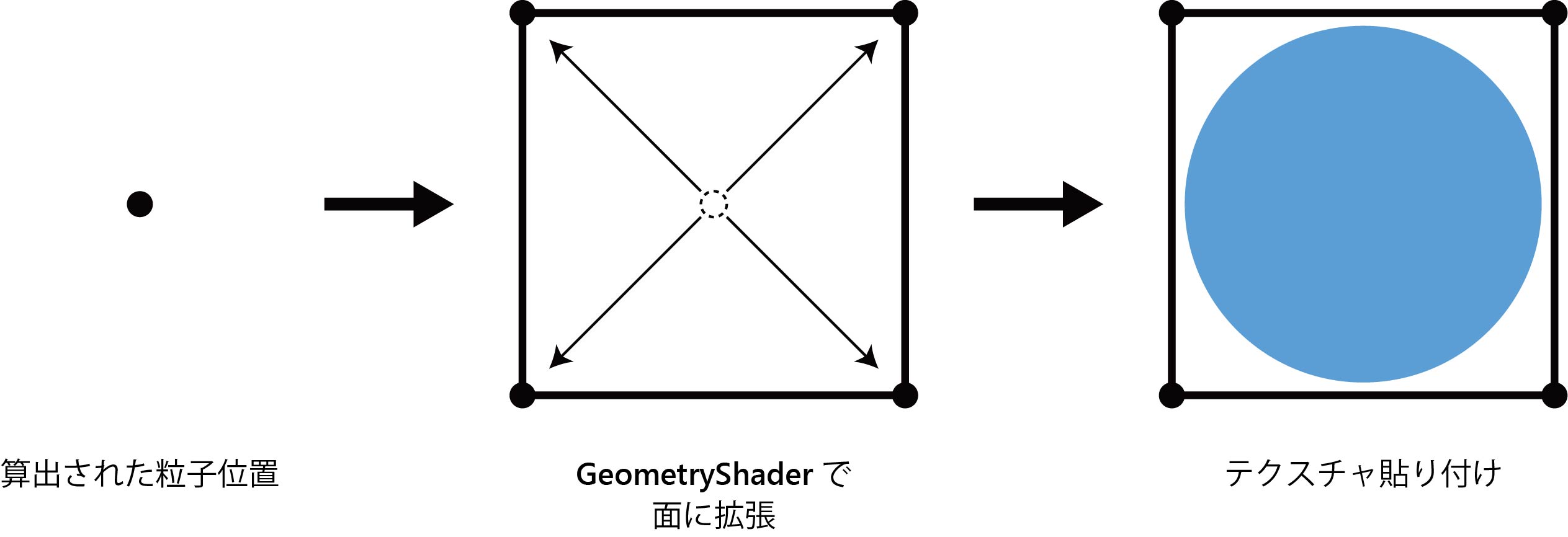
Figure 5.7: Creating a billboard
[* 10] A Plane whose table always faces the viewpoint.
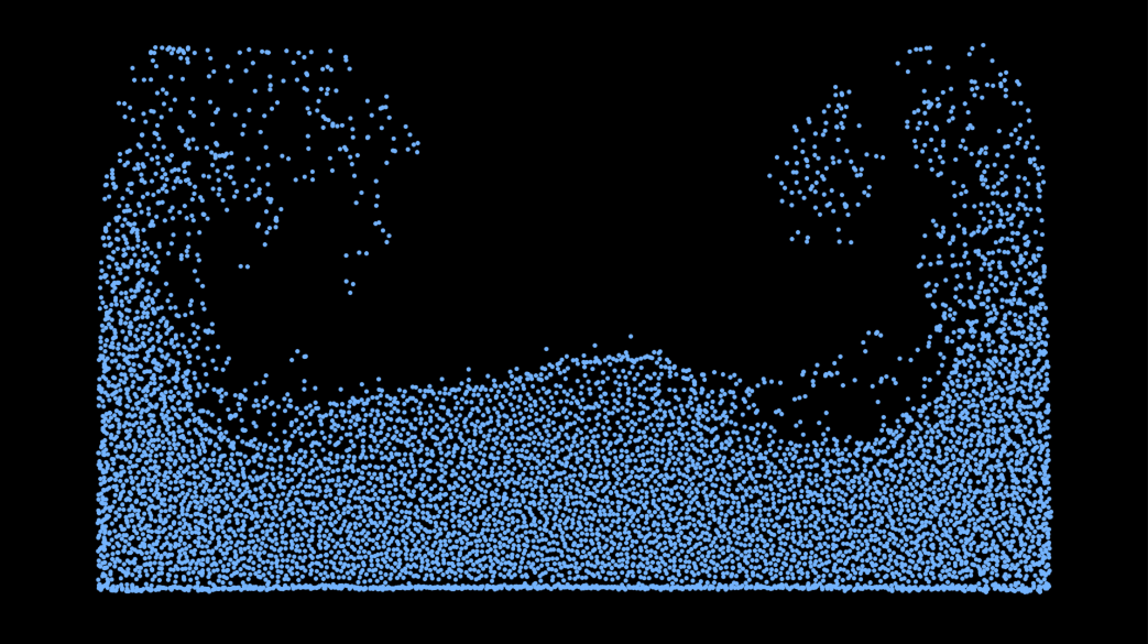
Figure 5.8: Rendering result
The video is posted here ( https://youtu.be/KJVu26zeK2w ).
In this chapter, the method of fluid simulation using the SPH method is shown. By using the SPH method, it has become possible to handle the movement of fluid as a general purpose like a particle system.
As mentioned earlier, there are many types of fluid simulation methods other than the SPH method. Through this chapter, we hope that you will be interested in other physics simulations themselves in addition to other fluid simulation methods, and expand the range of expressions.